Obtaining Contact Numbers using SMARTS

Because I'm on a roll with blogging right now and I am looking for excuses to not write the next paper, here is a post about how to utilize SMARTS[1] for something cheminformatically-vant such as the contact number[2]. We will base the new code on what I did in the last post I wrote. The contact number is basically "Select an $\alpha$-Carbon and count the number $\alpha$-Carbons within a sphere of a certain radius $R$ from it". This give rise to a 1D measurement (see below) of how buried residues are. If you massage your data enough (we will get to this in a later post) it can be used to validate whether a protein is folded (somewhat) correctly or not. There is much more to this story than I have room for on my blog, but I do recommend you follow the blog of Anders Christensen, a fellow student who folds more proteins than I.

Our work today shall start from Crambine (PDB: 1CRN) which I've prepared for your viewing pleasure in pymol

From last week, the boiler-plate code we shall start from is

import openbabel
filename = "1CRN.pdb"
pattern = "[$(CC(=O)[N,O])]"
obmol = openbabel.OBMol()
obpat = openbabel.OBSmartsPattern()
obconv = openbabel.OBConversion()
obconv.SetInFormat(filename[-3:])
obconv.ReadFile(obmol, filename)
obpat.Init(pattern)
obpat.Match(obmol)
alpha_carbons = [m[0] for m in obpat.GetUMapList()]

I'm interested in $\alpha$-Carbons so the atomic primitive pattern we use to match with will be

[$(CC(=O)[N,O])]

The last part, [N,O] is a match of either a Nitrogen or an Oxygen. This Oxygen match is needed for the C-terminal. Because we are using SMARTS, this is the only thing that will change in our code once it is done. Should we be interested in locating the carboxyl groups of the backbone for instance, simply change one pattern. Of course, if you want to match $\alpha$-Carbons to carboxyl groups, this requires an extra pattern match.

Running this code will return a list of atoms. To calculate the contact number, the following function iterates over each match, forms a pair with all other matches and calculates the contact number for one residue at a time

def ContactNumbersForCutoff(matches, rcut):
  contact_numbers = []
  for i in matches:
    contact_number = 0 
    ai = obmol.GetAtom(i)
    for j in matches:
      if i == j: continue
      aj = obmol.GetAtom(j)
      if ai.GetDistance(aj) < rcut:
        contact_number +=1

    contact_numbers.append(contact_number)
  return contact_numbers

which we will invoke to generate the list of contact numbers

cn12 = ContactNumbersForCutoff(alpha_carbons, 12.0)

Since I am fond of the matplotlib[3] library for python when dealing with plots and I don't feel like doing the hard work myself anyways, I'll just plot[4] the list of numbers using the following code

pylab.plot(cn12)
pylab.savefig("contact.png")

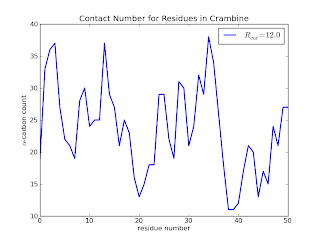
which (after some additional touches - see the github page for the final code) results in

Here we see that residues 20, 38, 39 and 40 are clearly not buried when compared to residues 30 to 36. In a later posts, I will add a few lines of code to calculate the above information in a slightly more useful way. I'd also like to explore a quick implementation of the Half-Sphere Exposure[5] method instead as it provides even more clue to the local environment.

check out the source code on my github page.