I wrote a post about adding a GUI to your command line interface program. Sometimes people just want to click stuff. If you tried it / implemented it yourself, you'd have seen that the program would have gone from responsive to non-responsive when you hit the run button. Why? Because the program can only do ONE think at a time and frankly, keeping the controls available for clicking at all times, updating the graphics and calculating particle movement do not get along nicely. This post is about making it behave like we expect.
I present to you threading. Specifically for PyQt there is the QThread class which is actually discussed rather nicely in this PyQtWiki and this page by Jo Plaete which I used for inspiration.
What complicates the whole scene is that we need to realize that we have two independant things we want to accomplish: 1) move particles and 2) update the graphics. Both independent of the GUI.
I started by making my own class called BaseThread which subclasses QThread. The code is
where I believe the magic for everything not just crashing and burning is the subtle use of the custom boolean flag exiting (which we will use later) and the use of self.wait() in the __del__ method. Again, for details you should read the blog posts mentioned above.
To come around many of the syncronization problems that arises with threads the Qt framework allows us to use custom signals to make everything talk together. Here is my version of a StepThread which defines the run method (you do NEVER call this explicitly!) and a convenience function called simulate to start a simulation for N steps. The run function emits a custom signal and sleeps for a little while before simulating again.
Very similarly we have the DrawThread which emits a signal so we can update the matplotlib surface.
Notice that it updates less frequently. I have yet to figure out something clever in this regard.
Finally, I had to make some tweaks to the Simulator class (nothing very fancy) to hook up our custom signals.
What I need now is a video of it and maybe to implement some different potentials instead of only the non-interacting particles. Stay tuned.
The entire code can be downloaded from the latest gist I made.
Showing posts with label python. Show all posts
Showing posts with label python. Show all posts
Thursday, June 28, 2012


Sunday, June 24, 2012
Adding a PyQt GUI to your program
I am all in for command line interface (CLI) programs. I'll admit that. They work in terminals. You can run them without an X Server and usually option flags are easy to use and obvious*. But sometimes I'd like to just hit a button. Click and magic happens. No more 200 character command line statement to get the ball rolling. A good example of this is from my colleague Anders Christensen who made a graphical user interface (GUI) for the Phaistos program.
In this post, we'll take the first small steps towards actually making a GUI for a simulation to run the ideal gas in and not just watch some numbers printed in a terminal. I'll be using Qt4 and the PyQt4 bindings. If you have a fairly recent linux distribution, you can apt-get install yourself to success very fast. Remember to also install the Qt-Designer app so you visually can layout your controls.
We'll start out simple by constructing buttons, textedits and a frame. I use a regular QWidget for my main form. The end goal for a user is to push the 1) setup button to initialize particles and 2) push the run button and make the simulation run. The simulation (i.e. the particles) should be displayed in the frame via matplotlib. It looks like this

If you want the resulting simulator.ui code its listed as part the gist for this blog post.
To move on from here, there is a nifty little tool called pyuic4 which will convert your .ui file into a python class with the name Simulator_UI. I always just parse it down to a file called simulator_ui.py. The code is
The simulator_ui class contains the framework for the QWidget form we will be using. The most clever approach I could think of was to subclass the simulator_ui class to separate the "setting up the form" code with the "what happens when I push a button" code. The QWidget I'll use to represent the window the user will see and I call it Simulator. It imports the Simulator_UI class, subclasses it and sets up the GUI. The two buttons are hooked up to either initialize new particles or run for some steps
The bread and butter of this application is the ParticleCanvas. Its tailored to draw and move the particles around. Look at its code
You see that it subclasses the Canvas class which is my best bet on how one should make the code for fast blitting of a matplotlib canvas. A class which subclasses the Canvas class is only responsible for redrawing the actual plot (and do it fast). However, I would gladly appreciate comments of you have a better way to implement it
Finally, the code that makes it all run is just my main executable which is defined like this
The final result looks like this
 We now have a finished simulation GUI. However, the main problem is that the GUI and the simulation code is intimately hooked up so the GUI will freeze at some point. Fortunately, it leaves a new post on the horizon.
*I never understood anything of the find command, however.
In this post, we'll take the first small steps towards actually making a GUI for a simulation to run the ideal gas in and not just watch some numbers printed in a terminal. I'll be using Qt4 and the PyQt4 bindings. If you have a fairly recent linux distribution, you can apt-get install yourself to success very fast. Remember to also install the Qt-Designer app so you visually can layout your controls.
We'll start out simple by constructing buttons, textedits and a frame. I use a regular QWidget for my main form. The end goal for a user is to push the 1) setup button to initialize particles and 2) push the run button and make the simulation run. The simulation (i.e. the particles) should be displayed in the frame via matplotlib. It looks like this

To move on from here, there is a nifty little tool called pyuic4 which will convert your .ui file into a python class with the name Simulator_UI. I always just parse it down to a file called simulator_ui.py. The code is
$ pyuic4 simulator.ui > simulator_ui.py
The simulator_ui class contains the framework for the QWidget form we will be using. The most clever approach I could think of was to subclass the simulator_ui class to separate the "setting up the form" code with the "what happens when I push a button" code. The QWidget I'll use to represent the window the user will see and I call it Simulator. It imports the Simulator_UI class, subclasses it and sets up the GUI. The two buttons are hooked up to either initialize new particles or run for some steps
The bread and butter of this application is the ParticleCanvas. Its tailored to draw and move the particles around. Look at its code
You see that it subclasses the Canvas class which is my best bet on how one should make the code for fast blitting of a matplotlib canvas. A class which subclasses the Canvas class is only responsible for redrawing the actual plot (and do it fast). However, I would gladly appreciate comments of you have a better way to implement it
Finally, the code that makes it all run is just my main executable which is defined like this
The final result looks like this

*I never understood anything of the find command, however.
Thursday, May 3, 2012
Programming the Ideal Gas
You've heard about it before. Many times. It's a model system used a lot in chemistry. The Ideal Gas law: A system where the particles can be treated as non-interacting. How do you program such a system? What do you need to describe it? Given 1) the basic introduction covered by Prof. Jan Jensen in another lecture, and 2) the following assignment (notice it is part 2), here is what the students are supposed to do once this exercise is complete:
Try and code it for yourself or use it in a course you teach. The students do find it interesting, both in the form of "what do I need to tell the computer to make it do stuff?" and "oh - the particles do move!".
Disclaimer: This code is part of a course I help teach at the University of Copenhagen - just imagine you never saw python before.
- Take a box with dimensions $(-1<x<1$ and $-1<y<1)$.
- Make npart particles placed randomly in the right side of a box ($0<x<1$) but evenly from the top through the bottom
- Give the npart particles random velocities in both directions and make it so they can move in both the positive and negative direction.
- Move the particles around via the equation: $X_i^{n+1} = X_i^{n}+dt*dX_i^{n}$
- Keep them inside the box at all times.
- Plot the result.
The students start out with 1, 2 and 6 presented to them, both for inspiration and because they contain some subtle hints. The code is
One of the tricky parts is knowing "what is the i'th particle" because we need this information to update the system according to the equation above in point 4. Once you realize that you can access this information in the X, Y, dX and dY arrays as X[i] under a loop, then there is really no problem with that point either, for instance, to update all particles according to the equation in 4 in one go, we could write
Assigning a loop to iterate over the particles is not really troublesome, but understanding why is hard - even to explain it to yourself. A simple for-loop might not be the smartest thing to do, but I think it is the easiest one to go about and more importantly I often feel that many things can get lost in the whole numpy magic, especially for newcomers.
The next part is, that we should keep the particles inside the box at all times. The exercise has a little discussion about which version is the better, but in my opinion the particles should always be inside at all times. To keep them in, we ask whether a step (equation in point 4) in X and Y will result in the particle being outside the box and if that is the case, we reverse velocity that potentially brought the particle outside. We could use the following code to do that
The next part is, that we should keep the particles inside the box at all times. The exercise has a little discussion about which version is the better, but in my opinion the particles should always be inside at all times. To keep them in, we ask whether a step (equation in point 4) in X and Y will result in the particle being outside the box and if that is the case, we reverse velocity that potentially brought the particle outside. We could use the following code to do that
Inserting the above two snippets of code, under a loop over the number of steps we want to take, we finally end up with the code that simulates non-interacting particles in a container.
Disclaimer: This code is part of a course I help teach at the University of Copenhagen - just imagine you never saw python before.
Friday, April 20, 2012
The Wonders of Numpy
I originally envisioned this post to be somewhat of a wall of code which would show just how ugly you can actually write code that works (see the public gist for that) but without the checks to see that it does what I want it to do. I've been parsing text lately - a weird and wonderful combination of taking the molecular orbital (MO) coefficients of a calculation and transforming them into a new basis set to calculate spin-spin coupling constants. This involves reading the input file to get the basis set exponents of the uncontracted basis set and matching them with the corresponding MO coefficients and generate a new segmented contracted basis set.
In the table below we have a segmented basis set where the primitive gaussian type orbitals (PGTO) are combined into contracted gaussian type orbitals (CGTO). In this case, we have a basis set with three degrees of freedom (three CGTOs) down from five degrees of freedom (five PGTOs). Dark fields in the table shows coefficients whose value are larger than zero. Bright fields are zero.
So the PGTOs are obtained from the .mol file (I'm using Dalton for this) using the read_mol.py script found in the gist since it is used anyways to generate the new basis set. The CGTOs are obtained from an RHF calculation (see the hf.dal file in the gist) using the read_log.py script.
The problem with the design of a new basis set is to choose how many of the PGTOs to use in a CGTO, for instance, why choose three PGTOs in CGTO1? Since the number of PGTOs is not too overwhelming, I've gone ahead and made a general solution so I have the possibility to test all cases. The main problem then boiled down to: given an N x N matrix with zeros (notice that there are many zeros in this matrix), how do I overwrite subarrays (3 x 1 in this case) in Numpy so I can insert a specific number of coefficients to make CGTO1 from PGTO1 to PGTO3? and how to I make CGTO2 and CGTO3 couple with PGTO4 and PGTO5 using identity matrix inserted at the correct spot?
The trick is to make use of Numpys excellent (and very difficult) features known as boolean masking where a matrix filled with True or False will extract the corresponding values and one is able to assign to them. In the end, we need to remove excessive columns and I've found my head can do that easily by doing a transpose of the matrix, remove the unneeded rows (using a simpler Numpy/python logic which I know by hand) and transpose it back.
This was one of the more difficult issues, but at least I can now generate a multitude of basis set calculations and examining my property of interest in a matter of seconds. Numpy rocks, but I think I could grow old trying to learn all the awesome features it has.
In the table below we have a segmented basis set where the primitive gaussian type orbitals (PGTO) are combined into contracted gaussian type orbitals (CGTO). In this case, we have a basis set with three degrees of freedom (three CGTOs) down from five degrees of freedom (five PGTOs). Dark fields in the table shows coefficients whose value are larger than zero. Bright fields are zero.
| CGTO1 | CGTO2 | CGTO3 | |
|---|---|---|---|
| PGTO1 | |||
| PGTO2 | |||
| PGTO3 | |||
| PGTO4 | |||
| PGTO5 |
So the PGTOs are obtained from the .mol file (I'm using Dalton for this) using the read_mol.py script found in the gist since it is used anyways to generate the new basis set. The CGTOs are obtained from an RHF calculation (see the hf.dal file in the gist) using the read_log.py script.
The problem with the design of a new basis set is to choose how many of the PGTOs to use in a CGTO, for instance, why choose three PGTOs in CGTO1? Since the number of PGTOs is not too overwhelming, I've gone ahead and made a general solution so I have the possibility to test all cases. The main problem then boiled down to: given an N x N matrix with zeros (notice that there are many zeros in this matrix), how do I overwrite subarrays (3 x 1 in this case) in Numpy so I can insert a specific number of coefficients to make CGTO1 from PGTO1 to PGTO3? and how to I make CGTO2 and CGTO3 couple with PGTO4 and PGTO5 using identity matrix inserted at the correct spot?
The trick is to make use of Numpys excellent (and very difficult) features known as boolean masking where a matrix filled with True or False will extract the corresponding values and one is able to assign to them. In the end, we need to remove excessive columns and I've found my head can do that easily by doing a transpose of the matrix, remove the unneeded rows (using a simpler Numpy/python logic which I know by hand) and transpose it back.
This was one of the more difficult issues, but at least I can now generate a multitude of basis set calculations and examining my property of interest in a matter of seconds. Numpy rocks, but I think I could grow old trying to learn all the awesome features it has.
Wednesday, January 18, 2012
Adding Hydrogen Atoms Is No Mean Feat
I've had a problem since Monday. Hydrogen atoms. You take an MD from say GROMACS or Tinker and make a 16 Angstrom extract of the entire system (this is Chorismate Mutase, PDB: 2CHT) in pymol via the command
so you can run QM/MM on it afterwards (see picture of the actual cut-out or look at my github page of the pdb-file with missing hydrogens).

However, doing the extract (which cuts the peptide-bond) improper chemistry appears around this bond since atoms are missing - on one side (where you remove atoms) it does not matter since you remove it all together, but on the side that remains, this is a big problem since the chemical valence is not correct. I want to add hydrogens where atoms are missing, but no standard solution was apparently available to add hydrogens to the bonds that were cut. Trying in pymol added hydrogens all over the place and the usual Open Babel tools also made funny business with the termini in its clever algorithms for proteins. In the end, it was time to revisit the good old trusty Open Babel and scour the API to actually see if something was usable. Again, I struck gold and here is what I did to actually make it work.

Chemically speaking, the local bonding environment is not satisfied at the points where cleavage took place. Open Babel has functionality to get the assumed valence of an atom as well as the actual valence (based on connectivity) - this we will use to our advantage and make sure it only applies to backbone carbons (not $C_{\alpha}$) and not to Oxygen.
For convenience I'm looping over residues and then atoms in residues and then seeing if the assumed and actual valencies are matching. This is not nescessary as I do not use any information about the residues (yet). If the valencies are not matching I add hydrogen(s) to the atom in question to satisfy the valency.
The following code does this
Notice it uses a new obutil.py module I've made with some convenience functions to easily access features of Open Babel. By using the code on the supplied model1.pdb file, one ends up with
and there you have it: A protonated cutout from an MD simulation which does not have reprotonated atoms.
NB! There is one issue with this approach which concerns the actual output to PDB. There is no reordering of the atoms when you save the file, so if you depend on the order of the atoms, then this approach needs some more work. A colleague (and I) have yet to figure out a clever way to actually do this.
cmd.select("sele", "(byres (sele expand 16))",enable=1)
so you can run QM/MM on it afterwards (see picture of the actual cut-out or look at my github page of the pdb-file with missing hydrogens).

However, doing the extract (which cuts the peptide-bond) improper chemistry appears around this bond since atoms are missing - on one side (where you remove atoms) it does not matter since you remove it all together, but on the side that remains, this is a big problem since the chemical valence is not correct. I want to add hydrogens where atoms are missing, but no standard solution was apparently available to add hydrogens to the bonds that were cut. Trying in pymol added hydrogens all over the place and the usual Open Babel tools also made funny business with the termini in its clever algorithms for proteins. In the end, it was time to revisit the good old trusty Open Babel and scour the API to actually see if something was usable. Again, I struck gold and here is what I did to actually make it work.

Chemically speaking, the local bonding environment is not satisfied at the points where cleavage took place. Open Babel has functionality to get the assumed valence of an atom as well as the actual valence (based on connectivity) - this we will use to our advantage and make sure it only applies to backbone carbons (not $C_{\alpha}$) and not to Oxygen.
For convenience I'm looping over residues and then atoms in residues and then seeing if the assumed and actual valencies are matching. This is not nescessary as I do not use any information about the residues (yet). If the valencies are not matching I add hydrogen(s) to the atom in question to satisfy the valency.
The following code does this
import sys
import openbabel
from obutil import *

if __name__ == "__main__":
  if( len(sys.argv) != 3 ):
    print "Usage: protonate in.pdb out.pdb"
    sys.exit()
  file_in = sys.argv[1]
  file_out = sys.argv[2]

  mol = OBMolFromFilename(file_in)
  for residue in openbabel.OBResidueIter(mol):
    rname = residue.GetName()
    chain = residue.GetChain()
    for atom in openbabel.OBResidueAtomIter(residue):
      if atom.IsCarbon() or atom.IsNitrogen():
        idx = atom.GetIdx()
        imval = atom.GetImplicitValence()
        reval = atom.GetValence()
        if imval != reval:
          print "%5i (%3s %s) %2i %2i" % (idx,rname,chain,imval,reval)
          mol.AddHydrogens(atom)

  OBMolToFilename(mol, file_out)
Notice it uses a new obutil.py module I've made with some convenience functions to easily access features of Open Babel. By using the code on the supplied model1.pdb file, one ends up with
    1 (VAL A)  3  2
    3 (VAL A)  3  2
   17 (ASP A)  3  2
  239 (LEU A)  3  2
  256 (PRO A)  3  2
  258 (PRO A)  3  2
  270 (VAL A)  3  2
  397 (THR A)  3  2
  409 (LEU A)  3  2
  808 (GLU A)  3  2
  821 (CYS A)  3  2
  910 (MET A)  3  2
  925 (GLY C)  3  2
 1008 (THR C)  3  2
 1020 (LEU C)  3  2
 1022 (LEU C)  3  2
 1039 (ILE C)  3  2
 1041 (ILE C)  3  2
 1058 (LEU C)  3  2
 1159 (LEU C)  3  2
 1176 (MET C)  3  2
 1450 (MET C)  3  2
 1465 (GLN C)  3  2
 1467 (GLN C)  3  2
 1482 (ILE C)  3  2
and there you have it: A protonated cutout from an MD simulation which does not have reprotonated atoms.
NB! There is one issue with this approach which concerns the actual output to PDB. There is no reordering of the atoms when you save the file, so if you depend on the order of the atoms, then this approach needs some more work. A colleague (and I) have yet to figure out a clever way to actually do this.
Wednesday, December 7, 2011
Obtaining Contact Numbers using SMARTS
Because I'm on a roll with blogging right now and I am looking for excuses to not write the next paper, here is a post about how to utilize SMARTS[1] for something cheminformatically-vant such as the contact number[2]. We will base the new code on what I did in the last post I wrote. The contact number is basically "Select an $\alpha$-Carbon and count the number $\alpha$-Carbons within a sphere of a certain radius $R$ from it". This give rise to a 1D measurement (see below) of how buried residues are. If you massage your data enough (we will get to this in a later post) it can be used to validate whether a protein is folded (somewhat) correctly or not. There is much more to this story than I have room for on my blog, but I do recommend you follow the blog of Anders Christensen, a fellow student who folds more proteins than I.
Our work today shall start from Crambine (PDB: 1CRN) which I've prepared for your viewing pleasure in pymol

Our work today shall start from Crambine (PDB: 1CRN) which I've prepared for your viewing pleasure in pymol

From last week, the boiler-plate code we shall start from is
import openbabel
filename = "1CRN.pdb"
pattern = "[$(CC(=O)[N,O])]"
obmol = openbabel.OBMol()
obpat = openbabel.OBSmartsPattern()
obconv = openbabel.OBConversion()
obconv.SetInFormat(filename[-3:])
obconv.ReadFile(obmol, filename)
obpat.Init(pattern)
obpat.Match(obmol)
alpha_carbons = [m[0] for m in obpat.GetUMapList()]
I'm interested in $\alpha$-Carbons so the atomic primitive pattern we use to match with will be
[$(CC(=O)[N,O])]
The last part, [N,O] is a match of either a Nitrogen or an Oxygen. This Oxygen match is needed for the C-terminal. Because we are using SMARTS, this is the only thing that will change in our code once it is done. Should we be interested in locating the carboxyl groups of the backbone for instance, simply change one pattern. Of course, if you want to match $\alpha$-Carbons to carboxyl groups, this requires an extra pattern match.
Running this code will return a list of atoms. To calculate the contact number, the following function iterates over each match, forms a pair with all other matches and calculates the contact number for one residue at a time
def ContactNumbersForCutoff(matches, rcut):
  contact_numbers = []
  for i in matches:
    contact_number = 0
    ai = obmol.GetAtom(i)
    for j in matches:
      if i == j: continue
      aj = obmol.GetAtom(j)
      if ai.GetDistance(aj) < rcut:
        contact_number +=1

    contact_numbers.append(contact_number)
  return contact_numbers
which we will invoke to generate the list of contact numbers
cn12 = ContactNumbersForCutoff(alpha_carbons, 12.0)
Since I am fond of the matplotlib[3] library for python when dealing with plots and I don't feel like doing the hard work myself anyways, I'll just plot[4] the list of numbers using the following code
pylab.plot(cn12)
pylab.savefig("contact.png")
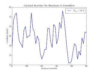
which (after some additional touches - see the github page for the final code) results in

Here we see that residues 20, 38, 39 and 40 are clearly not buried when compared to residues 30 to 36. In a later posts, I will add a few lines of code to calculate the above information in a slightly more useful way. I'd also like to explore a quick implementation of the Half-Sphere Exposure[5] method instead as it provides even more clue to the local environment.
check out the source code on my github page.
Wednesday, November 30, 2011
Cut'n'Frag: Fragment smart using SMARTS
In our research group, part of the research we do is method development. To facilitate these new methods, tools are often required to setup various calculations or treat output files. Some of this research[1] is in fragment based methods[2] where a large system is divided into several smaller pieces and the total property of the whole system can be assembled from the individual fragments.
To help facilitate easier setup of fragment based calculations, we've made a tool (still under development) called FragIt which we use to fragment large molecules and prepare input files for GAMESS[3]. This post is about one key aspect of FragIt: How to use Open Babel[4] to figure out where to cut bonds in a protein.
For starters, one needs to load a molecule from a file, this is accomplished by the following lines of code[*]
import openbabel
filename="1UAO.pdb"
obmol = openbabel.OBMol()
obconv = openbabel.OBConversion()
obconv.SetInFormat(filename[-3:])
obconv.ReadFile(obmol, filename)
which basically tells OpenBabel that we like to open a file with a fileformat specified by the extension of the filename("pdb").
Open Babel includes functionality to do SMARTS[5] pattern matching[6]. Basically, you write a pattern to search for a substructure in a molecule. The way we want to use it is to identify an atom A on one side of a bond, and an atom B on the other side of that bond. Thus, using the following SMARTS pattern on a protein
[$(CN)][$(C=O)]
we can search for A: 'find carbon connected to nitrogen on one side' and B: 'find carbon connected to an oxygen on the other side'. Results are only returned if the above pattern mathes on both sides of a bond at the same time. The code to do this is
obpat.Init(pattern)
obpat.Match(obmol)
matches = [m for m in obpat.GetUMapList()]
where the last line converts some horrible <openbabel.vectorvInt; proxy ... > SWIG code into a list of tuples with matching atom ID's, i.e.
print matches
gives
[(2, 3), (11, 12), (32, 33), (44, 45), (58, 59), (73, 74), (87, 88), (94, 95), (108, 109), (132, 133)]
Each tuple has information about the found atoms as (A, B).
The real beauty of this is of course that you can make your own patterns and match whatever you want in whichever molecule you chose to play with.
You can find this example as well as others on my github page.
[*] We opted for the full fledged API of OpenBabel, thus it takes 5 lines of code to actually open a file. The more pythonic library pybel[7] which is also included in OpenBabel was not used.
update: Thanks to Anders Christensen for pointing me towards an easy syntax highlighter.
Monday, October 31, 2011
Using OpenBabel to Make Input Files for GAMESS
One thing that people tend to hate to do, is to make repetitive tasks. One such thing could be to prepare 100 different geometry optimizations using DFT[1] and a happy mixture of basis sets[2] and functionals[3] for GAMESS[4]. In this blog post, I'll show you how you can get around manual labor and prepare 10 files with just a little bit of coding. Extending it to a 100 is an easy task after that. Lets start.
An input geometry of ethanol in the very common XYZ file format might look something very similar to this, when made in Avogadro[5]
Using Open Babel[6] we can quickly make a GAMESS input file using the following command
resulting in
but we can't run this file right away since it is obviously lacking information about the basis set, the DFT-functional and even the runtype (GAMESS assumes runtyp=energy if nothing is specified).
Ideally what we want is to generate a header for the input file and then insert it into the input file, but this header should be generated automatically for us.
Given a set of parameters (functional and basis set), the following python script (header.py) prints a correct header for GAMESS to the screen
Notice how we use a dictionary to store the basis set information so it can be easily recovered and printed correctly. The GAMESS basis group can be quite hideous with Pople basis sets[7].
All we require now is a small bash script, which makes loops over the various basis sets and functionals, invoke the python script we just made with the correct arguments and dump that printout information to a file (header.inp) and then use some Open Babel magic (to add a custom header with keywords, use the very secret -xf filename flag when converting to GAMESS input files) to make it work. The following script does exactly that
For information on how to use GAMESS, I recommend Professor Jan Jensens blog (http://molecularmodelingbasics.blogspot.com/) as a great resource and for general usage notes of GAMESS and the Google user group (http://groups.google.com/group/gamess) is very helpful if you have any problems or questions related to running GAMESS.
NB! To discover what options the babel file conversion tool supports for your file format (gamin in this case), simply invoke the following command
Happy Conversion!
An input geometry of ethanol in the very common XYZ file format might look something very similar to this, when made in Avogadro[5]
9
ethanol.xyz
C  0.00004  0.00001  0.00002
C  0.00035 -0.00106  1.52091
H  0.02794  1.04324 -0.38022
H -0.92039 -0.49540 -0.37524
H  0.88619 -0.55034 -0.38151
H -0.89666  0.55109  1.87908
O  1.16332  0.62487  1.98684
H -0.03205 -1.05436  1.87773
H  1.11207  0.59582  2.97727
Using Open Babel[6] we can quickly make a GAMESS input file using the following command
babel -ixyz ethanol.xyz -ogamin ethanol.inp
resulting in
 $CONTRL COORD=CART UNITS=ANGS $END
 $DATA
ethanol.xyz
C1
C 6.0  0.0000400000  0.0000100000  0.0000200000
C 6.0  0.0003500000 -0.0010600000  1.5209100000
H 1.0  0.0279400000  1.0432400000 -0.3802200000
H 1.0 -0.9203900000 -0.4954000000 -0.3752400000
H 1.0  0.8861900000 -0.5503400000 -0.3815100000
H 1.0 -0.8966600000  0.5510900000  1.8790800000
O 8.0  1.1633200000  0.6248700000  1.9868400000
H 1.0 -0.0320500000 -1.0543600000  1.8777300000
H 1.0  1.1120700000  0.5958200000  2.9772700000
 $END
but we can't run this file right away since it is obviously lacking information about the basis set, the DFT-functional and even the runtype (GAMESS assumes runtyp=energy if nothing is specified).
Ideally what we want is to generate a header for the input file and then insert it into the input file, but this header should be generated automatically for us.
Given a set of parameters (functional and basis set), the following python script (header.py) prints a correct header for GAMESS to the screen
import sys

basissets = {'sto3g' :'STO NGAUSS=3',
             'pc0' :'PC0',
             'pc1' :'PC1',
             'apc0' :'APC0',
             'apc1' :'APC1'}

functionals = {'blyp' :'BLYP',
               'b3lyp': 'B3LYP'}

basis = basissets[sys.argv[1]]
functional = functionals[sys.argv[2]]
print " $SYSTEM MWORDS=125 $END"
print " $CONTRL RUNTYP=OPTIMIZE DFTTYP=%s ISPHER=1 $END" % (functional)
print " $BASIS GBASIS=%s $END" % (basis)
Notice how we use a dictionary to store the basis set information so it can be easily recovered and printed correctly. The GAMESS basis group can be quite hideous with Pople basis sets[7].
All we require now is a small bash script, which makes loops over the various basis sets and functionals, invoke the python script we just made with the correct arguments and dump that printout information to a file (header.inp) and then use some Open Babel magic (to add a custom header with keywords, use the very secret -xf filename flag when converting to GAMESS input files) to make it work. The following script does exactly that
#!/usr/bin/env bash
for basis in sto3g pc0 pc1 apc0 apc1
do
  for functional in blyp b3lyp
  do
    filename=$basis"_"$functional".inp"
    python header.py $basis $functional > header.inp
    babel -xf header.inp -ixyz ethanol.xyz -ogamin $filename
  done
done
For information on how to use GAMESS, I recommend Professor Jan Jensens blog (http://molecularmodelingbasics.blogspot.com/) as a great resource and for general usage notes of GAMESS and the Google user group (http://groups.google.com/group/gamess) is very helpful if you have any problems or questions related to running GAMESS.
NB! To discover what options the babel file conversion tool supports for your file format (gamin in this case), simply invoke the following command
babel -H gamin
Happy Conversion!
Subscribe to:
Posts (Atom)